Notebooks Are Lying to You

Jupyter has a dirty secret, and it’s not that the interface is ugly. It’s that the notebook you’re looking at might not represent reality.

Say you’re analyzing sales data. Three cells:

# Cell 1
df = pd.read_csv("sales.csv")

# Cell 2
df = df[df["region"] == "North America"]

# Cell 3
df.groupby("product").revenue.sum()

You run them top to bottom. Numbers look right. You send the report.

Two days later your manager asks the same analysis for EMEA. You go back to cell 2:

# Cell 2 (edited)
df = df[df["region"] == "EMEA"]

You re-run cell 2 and cell 3. The numbers update. You send it.

The numbers are wrong.

Cell 2 didn’t run on fresh data. It ran on whatever df already was in memory. You filtered a filtered dataframe. It looks plausible. Nothing fails.

This is the best-case version of the problem, because at least you could catch it if you were careful. Here’s a worse one.

You’re cleaning up the notebook a week later. You decide cell 1 is redundant (the data loading now happens upstream) so you delete it. You re-run everything. It works. Of course it does: df is still alive in the kernel from the last run. You deleted the cell, not the variable. These are what I call ghost variables: they lurk in your kernel long after the cell that created them is gone.

For a solo analyst this is annoying but manageable. You wrote the code, you remember the order, you keep it in your head. But the moment someone else touches it, or you come back to it three days later, that implicit mental model breaks down fast. Whose state is the kernel in? Nobody knows.

There’s a second problem layered on top of this. In a standard notebook, if cell A defines df and cell B uses df, the relationship is implicit. Nothing in the cell metadata says “B depends on A.” You just know because you wrote it that way. This causes two specific failures in practice:

Stale reads. Alice modifies cell A and re-runs it. Cell B is now stale but still shows the old output. Bob is looking at B and has no idea it’s out of date.

Ordering drift. The cell order in the UI no longer matches the execution order that produced the current state. Notebooks accumulate hidden history. Running the notebook top-to-bottom stops meaning anything.

Jupyter has had an open issue about this since 2015.

The fix is dependency tracking. If the system knows B depends on A, it can automatically invalidate and re-execute B when A changes.

At Livedocs this was worse, because I wasn’t just dealing with Python cells. Last time I counted there were 10 cell types. A chart renders a dataframe. That dataframe comes from a SQL query. That query references a Python variable. That variable was defined three cells up.

If I had to draw that on a whiteboard, my brain automatically draws a graph. Cells are nodes. The “this feeds into that” relationships are edges.

A Directed Acyclic Graph is the right structure for this. The hard part was building one automatically, without asking users to draw it themselves.

Notebook == Graph?

The first question is how to actually build a graph from a notebook. Every cell type needs to expose the same two things: what names it produces, and what names it consumes.

Take a cell:

y = x + 1

You can describe it completely with:

yields:       y
dependencies: x

Now do that for every cell. If one cell yields x and another depends on x, draw an edge. The graph builds itself.

I call these yields and dependencies. The key insight that made this tractable for all 10 cell types: every cell in Livedocs, regardless of what it looks like to the user, gets compiled down to a Python snippet before execution.

A SQL cell with Jinja templating like SELECT * FROM {{ df }} becomes Python that renders the template, runs the query, and assigns the result to a variable. A chart cell becomes a Python call that reads a dataframe and renders graphics using Vega. An input control becomes a variable assignment. They all use the same Python SDK that gets loaded into the kernel.

So you only need to solve one problem: given a Python snippet, what names does it define, and what names does it read from? Get that right and the dependency graph falls out naturally.

Walking the AST

To extract yields and dependencies from a cell, I parse the Python AST and walk it. I did this in Rust using rustpython-parser, primarily because this runs on every keystroke and needed to be fast + it fits in well with rest of the execution cycle.

struct AstVisitor {
    yields: HashSet<String>,
    dependencies: HashSet<String>,
    yield_types: HashMap<String, String>,
    bound: HashSet<String>,  // names defined so far in this cell
    in_loop_target: bool,
    in_with_vars: bool,
}

The bound set is the key mechanism. As the visitor walks the cell top to bottom, every name it assigns goes into bound. When it encounters a name being read, it only registers it as a dependency if it’s not already in bound. That’s the entire free variable analysis.

fn visit_expr_name(&mut self, node: ExprName) {
    let name = node.id.to_string();
    if node.ctx.is_store() {
        self.bound.insert(name.clone());
        self.yields.insert(name);
    } else if node.ctx.is_load() {
        if !self.bound.contains(&name) {
            self.dependencies.insert(name);
        }
    }
}

So if a cell does:

x = 10
y = x + 1

x enters bound on the first line. When the visitor sees x being read on the second line, it’s already in bound, so it doesn’t become a dependency. The cell is self-contained. x and y are both yields, nothing is a dependency.

But if a cell does just:

y = x + 1

x is read before it’s ever assigned. It’s not in bound. It becomes a dependency — something another cell needs to have produced.

The footguns

Simple name loads and stores are easy. The interesting cases are where Python’s evaluation semantics create traps.

Augmented assignment. x += 1 is both a read and a write. If x doesn’t already exist somewhere, this line errors. The visitor handles this by checking the bound state before visiting the target:

fn visit_stmt_aug_assign(&mut self, node: StmtAugAssign) {
    let is_target_bound = match node.target {
        Expr::Name(name) => self.bound.contains(&name.id),
        _ => false,
    };

    self.visit_expr(node.value);   // visit RHS first
    self.visit_expr(node.target);  // adds name to yields/bound

    if !is_target_bound {
        // x wasn't defined in this cell before this line, so it's a dep
        self.dependencies.insert(name);
    }
}

RHS before LHS. Regular assignments also visit the value before the target. This matters for patterns like df = df.head(10). The read of df on the right happens before the write on the left, so df correctly becomes a dependency even though it’s also a yield.

For loop ordering. for x in items — the iterator items is a dependency, x is a yield. The visitor visits the iterator expression first, then the target, so for x in x (where you iterate over a variable with the same name as the loop variable) correctly registers the outer x as a dependency.

fn visit_stmt_for(&mut self, node: StmtFor) {
    self.visit_expr(node.iter);    // iterator first — free variable

    self.in_loop_target = true;
    self.visit_expr(node.target);  // then the loop variable
    self.in_loop_target = false;

    for stmt in node.body {
        self.visit_stmt(stmt);
    }
}

Function bodies. The visitor runs with module_only: true for all normal notebook analysis. When it hits a function definition, it walks the decorators (which execute at definition time) but skips the body entirely. Names inside a function body don’t leak to module scope, so they shouldn’t become dependencies or yields of the cell.

fn visit_stmt_function_def(&mut self, node: StmtFunctionDef) {
    if self.config.module_only {
        for decorator in node.decorator_list {
            self.visit_expr(decorator);  // decorators run at definition time
        }
        // body is skipped — not module-level
    }
}

Comprehension variables. [i for i in items] — i is scoped to the comprehension in Python 3, so it should never become a cell-level yield. The visitor deliberately skips comprehension targets:

fn visit_comprehension(&mut self, node: Comprehension) {
    // do not visit node.target — comp vars don't leak to module scope
    self.visit_expr(node.iter);
    for condition in node.ifs {
        self.visit_expr(condition);
    }
}

This is slightly inaccurate to Python’s actual semantics in edge cases, but it’s what the tests encode — and in practice it doesn’t matter, because notebook cells that depend on comprehension variables being in scope are rare to the point of nonexistent.

Normalizing cell types

The visitor produces a ParserResult = (Yields, Dependencies). Every cell type normalizes to this same shape:

fn parse_cell(&mut self, cell_id, src, cell_type, datasource) -> ParserResult {
    match cell_type {
        Python        => parse_python(src, cell_id),
        Sql           => parse_sql(src, cell_id, datasource),
        Text          => parse_jinja(src, cell_id),
        Prompt        => parse_prompt(src, cell_id),
        Chart | Table => parse_datasource(datasource, cell_id),
        Input         => parse_input(src, cell_id),
        Canvas        => parse_canvas(src, cell_id),
        ...
    }
}

Chart and Table cells don’t have freeform source code — their only dependency is whichever dataframe/database they’ve been pointed at via the UI. parse_datasource just reads that configuration and returns it as a dependency.

SQL cells are interesting. They can’t yield anything in the traditional sense — a SQL query doesn’t define a Python variable. But the engine auto-generates a dataframe name for each SQL cell and injects it as a yield. The dependencies come from two sources: Jinja template variables in the query body ({{ df }}), and the datasource configuration (which might itself reference a dataframe produced by another cell).

Prompt cells are just parse_jinja called twice — once on the system instruction, once on the user prompt — with the results merged.

Everything flows into the same graph construction logic.

Building the DAG

The graph is a DiGraph (directed graph) from petgraph, with cells as nodes and DataField structs as edge weights. Each DataField carries the variable name, its inferred type, its producer’s cell ID, and a reference count.

The key design decision is how dependencies bind to producers. The rule is: a dependency binds to the nearest prior yield in editor order, and only to a prior yield. Forward references stay unbound. This is what prevents false cycles and keeps the graph acyclic by construction in the normal case.

The full edge set is rebuilt from scratch on every structural change — a cell edit, a deletion, a reorder. No incremental patching. This sounds expensive but it’s a single O(n) pass over the cells; the rebuild is just pointer operations. Re-parsing only happens when a cell’s source actually changes.

fn rebuild_all_edges(&mut self) {
    self.graph.clear_edges();

    let ordered_ids = match &self.editor_grid {
        Some(grid) => self.linearize_editor_grid_order(grid),
        None => self.graph.node_indices().map(|idx| self.graph[idx].id).collect(),
    };

    let mut last_def: HashMap<String, NodeIndex> = HashMap::new();

    for cell_id in ordered_ids {
        let node_idx = id_to_index[&cell_id];

        // For each dependency this cell has, bind to nearest prior definition
        for dep_name in node.dependencies.keys() {
            if let Some(&producer_idx) = last_def.get(dep_name) {
                dep.cell_id = graph[producer_idx].id;
                graph.add_edge(producer_idx, node_idx, dep);
            }
            // If not in last_def, dependency stays unbound — no edge added
        }

        // Register this cell's yields as definitions for subsequent cells
        for name in node.yields.keys() {
            last_def.insert(name, node_idx);
        }
    }

    self.recompute_reference_counts();
}

The traversal is a single linear pass in editor order, maintaining a last_def map. Each cell’s dependencies are resolved against whatever last_def currently says for that name. Then the cell’s own yields update last_def for future cells.

This means if two cells both yield df, the second one wins. Cells after it bind to the second definition. Cells between the two bind to the first. It’s predictable and it matches how people actually think about notebooks — the most recent assignment is the one that’s live.

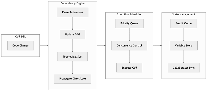
Reordering cells changes the dataflow

When a user drags a cell to a new position, the engine calls set_editor_grid(). Before rebuilding, it snapshots the current dependency bindings for every cell. After rebuilding with the new order, it compares:

fn set_editor_grid(&mut self, grid: EditorGrid) {
    // Snapshot current bindings
    let old_bindings: HashMap<CellId, HashMap<String, CellId>> =
        self.graph.node_weights()
            .map(|node| {
                let bindings = node.dependencies.iter()
                    .map(|(k, v)| (k, v.cell_id))
                    .collect();
                (node.id, bindings)
            })
            .collect();

    self.editor_grid = Some(grid);
    self.rebuild_all_edges();

    // Mark dirty any cell whose producer changed
    let changed: Vec<CellId> = self.graph.node_weights()
        .filter(|node| {
            let old = &old_bindings[&node.id];
            node.dependencies.iter().any(|(k, v)| old.get(k) != Some(&v.cell_id))
        })
        .map(|node| node.id)
        .collect();

    for id in changed {
        self.mark_dirty(&id);
    }
}

If moving cell A past cell B changes which producer cell C’s df dependency binds to, cell C gets marked dirty automatically. The user moved a cell and the system figured out what else changed. That’s the reactive part of having a graph instead of just an execution order.

Dirty marking and reactive execution

When a cell’s source changes, everything downstream gets marked dirty. Dirty cells show a visual indicator so you know at a glance which parts of the notebook are out of sync with what’s currently in the kernel. They re-execute the next time you run the notebook.

The propagation is a DFS over the downstream subgraph:

fn mark_dirty(&mut self, cell_id: &CellId) -> Vec<CellId> {
    let node_index = self.get_node_index(cell_id);
    let mut dirty_cells = Vec::new();

    let mut dfs = Dfs::new(&self.graph, node_index);
    while let Some(nx) = dfs.next(&self.graph) {
        let node = &mut self.graph[nx];
        if !node.dirty {
            node.dirty = true;
            dirty_cells.push(node.id);
        }
    }

    dirty_cells
}

Dirty is cleared when a cell successfully re-executes:

fn update_cell_output(&mut self, cell_id: &CellId, result: &RunResult) {
    let node = self.get_node_mut(cell_id);
    node.result = Some(result);
    node.dirty = false;
}

One thing worth noting: there’s no output-hash optimization that short-circuits propagation if a cell’s output didn’t meaningfully change. The propagation is purely structural. If you’re upstream of ten cells and your output changes, all ten get marked dirty and will re-execute. For most notebooks this is fine. For deeply chained notebooks with expensive computations it’s a real cost, and something I’d want to address in a future version.

Cycles are where things get sketchy

petgraph’s toposort returns an error if it finds a cycle. When that happens, the engine falls back:

fn topological_sort(&self, graph: &DiGraph<Cell, DataField>) -> ExecutionOrder {
    match toposort(graph, None) {
        Ok(order) => order.iter().map(|&idx| graph[idx].id).collect(),
        Err(_) => {
            // Log which cells form the cycle using Kosaraju SCC
            let sccs = kosaraju_scc(graph);
            for group in &sccs {
                if group.len() > 1 {
                    let cycle_ids: Vec<String> = group.iter()
                        .map(|&idx| graph[idx].id)
                        .collect();
                    error!("Cycle detected: {:?}", cycle_ids);
                }
            }

            // Fall back to editor order
            graph.node_indices().map(|idx| graph[idx].id).collect()
        }
    }
}

I did look into a smarter solution. Strongly Connected Components let you find all the cells involved in a cycle, then collapse each cycle into a single atomic node via edge contraction. A graph of SCCs is always a DAG — you’ve mathematically removed the cycles. You could then execute the collapsed SCC as a unit.

I didn’t ship it. The problem is what “execute as a unit” actually means for the user. It means running a set of cells in some order the system chose, mutating shared state in ways nobody asked for. The whole point of the DAG was to make execution deterministic and predictable. Collapsing SCCs trades one kind of surprise — an error — for a worse kind: silent unexpected executions. The fallback to linear editor order is less clever, but it’s not a surprise. The user gets the behavior they’d expect from any regular notebook.

Deletion and ghost variable cleanup

When a cell is deleted, the engine needs to clean up its variables from the kernel. Otherwise the ghost variables I mentioned earlier just keep lurking — making other cells work when they shouldn’t, or causing confusing behavior when a new cell reuses the same name.

The cleanup looks at what the deleted cell yielded, then checks whether any other cell also yields those same names:

async fn remove_cell(&mut self, cell_id: &CellId) {
    let node = self.dag.get_node(cell_id);

    // Find variables yielded by this cell
    let names_to_check: Vec<String> = self.yields.iter()
        .filter(|(_, field)| field.cell_id == *cell_id)
        .map(|(_, field)| field.name)
        .collect();

    for name in names_to_check {
        // Only delete if no other cell also yields this name
        let is_redeclared = self.dag.get_nodes().iter()
            .filter(|n| n.id != *cell_id)
            .any(|n| n.yields.contains_key(&name));

        if !is_redeclared {
            kernel.execute(format!("if '{}' in globals(): del {}", name, name)).await;
        }
    }
}

The rule is: if this name is yielded by any other cell in the graph, leave it alone — another cell owns it now. If nobody else yields it, evict it from the kernel.

One non-obvious detail: reference_count is tracked on each yield and recomputed after every graph rebuild, but it’s not what drives the cleanup decision. The cleanup uses a live redeclaration scan instead. The refcount exists for the LSP to surface information about what’s actively being used, not for deletion logic.

Cell updates work similarly — when a cell’s source changes and it no longer yields a variable it used to, the old variable gets evicted from the kernel before the new code runs. No ghost state survives an edit.

From static analysis to runtime values

The visitor produces sets of names. But a SQL cell with {{ df }} in its query doesn’t just need to know that df is a dependency — at execution time it needs the actual value of df so the Jinja template can render.

The transformer bridges this. When a SQL cell is about to execute, it generates a context-building snippet that walks the dependency list and evals each name into a dict:

_livedocs_{cell_id}_ctx = {}
deps = json.loads("{serialized_dependencies}")

for dep_name in deps:
    try:
        _livedocs_{cell_id}_ctx[dep_name] = eval(dep_name)
    except:
        raise Exception(f"Unable to find {dep_name} — make sure the cell that defines it has been run")

This runs before the SQL query itself. Whatever df currently is in kernel scope gets dropped into the context dict. The Jinja template then renders against that dict. Static analysis told the engine that df is a dependency. This is how that fact becomes a runtime value.

SQL cells also synthesize two variables on output — df and df_yielded:

df, df_yielded = livedocs.query(
    query="""SELECT * FROM {{ df }}""",
    datasource="...",
    context=_livedocs_{cell_id}_ctx,
    use_cache=True,
    ...
)
df_yielded  # surface the result

df is the actual dataframe. df_yielded is what gets shown in the cell output. The DAG tracks df as the yield. The split exists so you can use df downstream while the cell still displays results correctly.

What it unlocks

The LSP gets its state from the DAG. Every cell is a document in the Language Server Protocol sense, and the DAG is the authority on what names are defined and where. When a cell is deleted, the LSP immediately knows that cells downstream of it are referencing a name that no longer has a producer. The error surfaces before anyone runs anything.

SQL caching piggybacks on dirty state. Livedocs follows a push-down compute model — if a query runs against a warehouse, the engine lets the warehouse execute it and returns the result as a Polars dataframe. If none of the cells feeding into a SQL cell are dirty, it serves the cached result instead of re-querying the provider. For expensive queries against big tables, this makes a real difference in how fast the notebook feels to use.

The collab layer

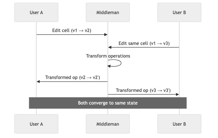
The design was straightforward on paper: operational transforms handle the user-facing conflict resolution — concurrent typing, cell ordering, simultaneous edits to the same cell. The DAG handles execution scheduling. When an OT merge resolves and a cell’s source changes, the DAG re-analyzes it and schedules downstream re-execution automatically. Two people editing cells in different parts of the dependency graph can work simultaneously without any coordination. Two people editing cells in the same dependency chain get their changes serialized through the DAG, which picks up from the last consistent state.

I built most of it, but didn’t ship it for three reasons.

First: this works great for Python or SQL or anywhere text appears, but what does it even look like to collaboratively edit a Chart? And why would anyone want to do that?

Second: global cell locking (one person executes at a time) was simpler and good enough for how people actually used the product.

Third, and most interesting: after I released the Livedocs agent, most users stopped writing cells at all. The agent was generating the notebook for them. Investing further in collaborative cell editing didn’t make sense when cells weren’t being manually authored anymore.

Where it breaks down

The AST approach works well for typical data science code. It struggles in a few places:

Dynamic attribute access. getattr(obj, name) where name is a runtime variable. No static analysis can know what that resolves to.

exec() and eval(). Treated as completely opaque. No dependency inference across them.

Mutating shared objects. The DAG tracks variable names, not object identity. If two cells hold a reference to the same mutable dataframe and both modify it without reassigning the variable, the dependency won’t be captured. This is a real limitation for imperative patterns.

Function body dependencies. The visitor runs with module_only: true, which means it skips function bodies entirely. If you define def f(): return df in a cell, the DAG has no idea that cell depends on df. The tradeoff was intentional — function-internal names shouldn’t leak to module scope — but it means cells that wrap logic in functions are effectively opaque to the dependency engine.

Shallow type inference. yield_types only gets populated for single-target constant assignments — x = 1 gives you int, x = "hello" gives you str. Anything more complex comes back as unknown. This matters because type information is used downstream by the LSP to surface better hints. In practice most notebook variables are dataframes or computed values, so unknown is the common case.

No output diffing. When a cell re-executes, the dirty propagation is purely structural. If a cell’s output didn’t actually change — same dataframe, same values — all downstream cells still get marked dirty and re-execute anyway. For long chains with expensive computations this adds up.

I considered a manual override: explicit dependency declarations for when inference gets it wrong. Never made it to prod because the UX is annoying, and in practice static analysis caught enough that manual wiring wasn’t necessary.

The DAG was just the start

The DAG turned out to be more useful than I originally planned for. It started as a fix for the hidden state problem and execution order mishaps. It became the foundation for the LSP integration, the SQL caching layer, and ghost variable cleanup. When I built the agent, the graph was already there. The agent could read it to understand the notebook’s structure, figure out which cells to modify, and insert new cells without breaking existing dependencies.

That part of the story is a post for another day.